The impact of network topological structures on systematic technology adoption and carbon emission reduction – Scientific Reports

Editor2

October 14, 2021

The impact of network topological structures on systematic technology adoption and carbon emission reduction – Scientific Reports

[ad_1]

In this section, we assume that there are 1000 nodes in the network (i.e., 1000 agents in the entire system). One of the agents (let it be Agent 1) holds the technological lead in the new advanced technology, which means, it has already possessed some knowledge and experience of T3. Naturally, Agent 1 will adopt T3 earlier than the other agents and act as the leader in the network. Other 999 agents are thus the followers in the network. Each agent makes technology adoption decisions with the optimization model introduced in the previous section, and each agent also adopts the ‘moving window’ limited foresight decision scheme with the same foresight of 50 years, which follows previous literature³³. The decision horizon is 100 years. Other initial parameters for all the agents are the same (as shown in Table S1 in the Supplementary Methods), except that for Agent 1, (overline{x}_{3}^{0} = 50). The settings of the parameters’ initial values also follow previous researches²⁹. The simulation settings are deliberately simplified so that we can observe more transparently how the new advanced technology diffuses from the leader to the followers in the network with different topological structures. It should be noted that, in our model, each technology essentially represents a cluster of related technologies with the infrastructure being in the center. The diffusion of a cluster of new technology can span up to a century . It takes even a longer time to evaluate the climate impact of a new technology. Therefore, we set the simulation time to 100 years.

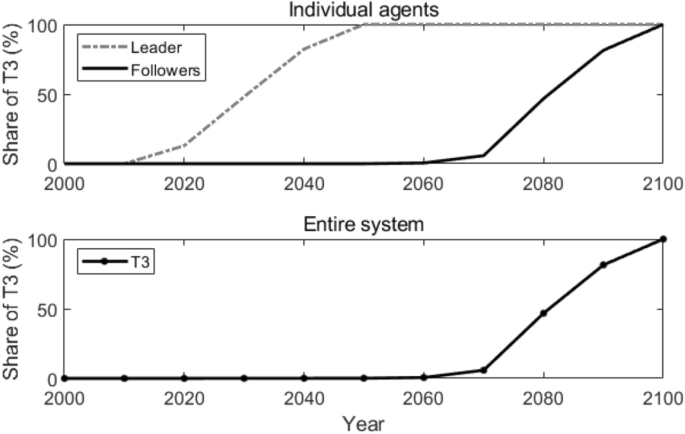
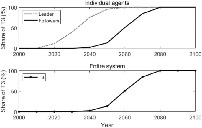
Figure 1 shows how T3 is adopted by the leader (Agent 1) and the followers (other agents) individually in the reference scenario when all the agents make decisions independently without exchanging any information or knowledge with each other, i.e., there’s no technological spillover among agents. Since the leader holds the technological lead in the new advanced technology T3, it adopts T3 around the year 2020, while the followers adopt T3 around the year 2080 (when the share of T3 reaches 10%). How the new advanced technology T3 is adopted in the entire system is also shown in Fig. 1. Due to the fact that the followers take up the overwhelming majority number of all the agents, T3’s adoption in the entire system seems the same as the followers, which is around the year 2080.

The no-spillover scenario can also be viewed as the investment failure scenario, since the followers cannot acquire the knowledge of the new technology from the leader and continue to use the old technology until the new technology becomes cost-effective for them. In the following simulations, we assume that the technological spillover effect exists among the agents. We will investigate how T3 diffuses from the leader to the followers when the technological spillover network is a regular lattice, a random network, or a scale-free network, respectively.

Regular lattices

Globally coupled network

In a globally coupled network, all nodes are connected with each other, as illustrated in the left panel of Fig. 2, taking a network with 10 nodes as an example.

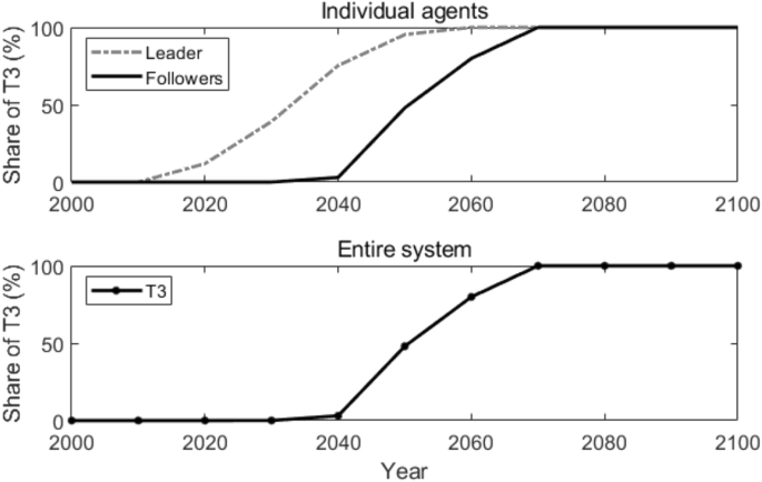
Since all the 1000 agents in the network are connected with each other, every follower agent acquires the same information at each time t, and thus makes the same technology adoption decisions. Figure 3 shows how T3 is adopted by the leader and the followers individually and in the entire system. Compared with the results in the reference scenario, T3 is adopted 30 years earlier by the followers and in the entire system in the globally coupled network.

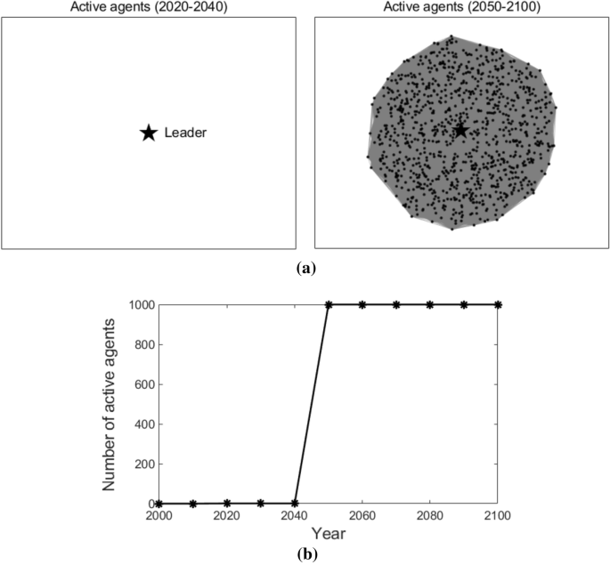
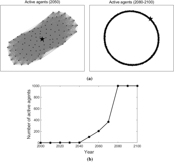
Figure 4 illustrates the agents in the network who adopt T3 at different times (as shown in Fig. 4a), agents who do not adopt T3 are removed from the figures) and the number of agents that adopt T3 at different times (as shown in Fig. 4b)). To make the description clearer, agents who adopt T3 at time t are named active agents at time t. The leader is highlighted with a star-shaped node, while the followers are represented with dot nodes. The edges among the nodes are shown with grey lines in the figures, which represent the connections among agents. As we can observe in Fig. 4, in the early stage (2000–2010), no agent adopts T3; from the year 2020 to 2040, only the leader adopts T3; after the year 2050, all the followers start to adopt T3. This is because, in a globally coupled network, all the followers are connected to the leader and with each other. Therefore, they adopt the new advanced technology at the same time.

Nearest-neighbor coupled network

In a nearest-neighbor coupled network, each node only connects with its K neighbor nodes (K/2 neighbor nodes on each side), as illustrated in the middle panel of Fig. 2, taking 10 nodes and K = 4 as an example.

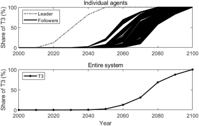
In our simulation, we let K = 100, which means each agent connects with its 100 neighbor agents (50 neighbor agents on each side). Figure 5 shows how T3 is adopted by each individual agent and in the entire system. The followers adopt T3 gradually since they acquire the knowledge of the new advanced technology at different times. The earliest and the latest adoption of T3 for the followers are around the years 2050 and 2080. There is an adoption time lag of 30 years among the followers. In the entire system, T3 is adopted around the year 2060, 20 years earlier compared with the results in the reference scenario.

Figure 6 illustrates the active agents at different times (as shown in Fig. 6a) and the number of active agents that changes over time (as shown in Fig. 6b) in the nearest-neighbor coupled network. The star-shaped node also represents the leader, and the dot nodes also represent the followers. As we can observe, in 2050, not many followers adopt T3. After that, more and more followers start to adopt T3 and the number of active agents keeps increasing. After the year 2080, T3 is adopted by all the agents. This is because, in a nearest-neighbor coupled network, each agent connects with its neighbor nodes. Followers can only acquire the knowledge of T3 gradually from its neighbors. As a result, the number of active agents also increases gradually.

Star coupled network

In a star coupled network, there is one node that occupies the center of the star and all the other nodes only connect with the center node, as illustrated in the right panel of Fig. 2, taking 10 nodes as an example.

In our simulation, Agent 1 has the technological lead, therefore, it is assumed intuitively to be the center node, and all the followers connect with and only with it. As a matter of fact, since all the followers are identical and only connect with the leader, they also acquire the same knowledge at each time t, and thereby make the same technology adoption decisions as well. Figure 7 shows how T3 is adopted by the leader and the followers individually and in the entire system. Compared with the results in the reference scenario, T3 is adopted 30 years earlier by the followers and in the entire system.

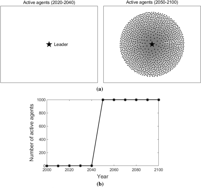
Figure 8 illustrates the active agents at different times and the number of active agents that changes over time in the star coupled network. From the year 2020 to 2040, only the leader adopts T3. After the year 2050, all the followers start to adopt T3. This is because, in a star coupled network, the followers only connect to the leader and can acquire the knowledge of T3 directly from the leader. Therefore, similar to the globally coupled scenario, they adopt T3 quickly and at the same time.

Random networks

In this subsection, we will run simulations under the assumption that the technological spillover network among all the 1000 agents is a random network. We follow the study conducted by Erdős and Rényi to construct the ER random graph (G_{N,p}^{ER}), where each pair of nodes is assumed to be connected with a probability p³⁵. To capture its dynamics, we also assume that the static random networks among all the nodes are different at different times.

According to the random graph theory, suppose that there are N nodes in a network, there is a critical probability (p_{c} = 1/N). Also, when (p ge {text{ln}}left( N right)/N), almost any graph in the ensemble (G_{N,p}^{ER}) is totally connected^35,36. Therefore, in our research, we will run different simulations with the connecting probability p equals to 0.001, 0.01, and 0.1, respectively. We will explore how the new advanced technology diffuses in the randomly connected networks in the following three scenarios: (a) when the connecting probability is comparatively low; (b) when there exists a giant component in the network; and (c) when the random network is always connected.

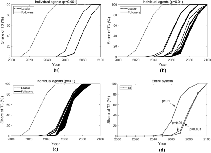
Figure 9 shows how T3 is adopted by each individual agent (sub-figures (a), (b) and (c), in which the dashed line represents the leader and the solid lines represent the followers) and in the entire system (sub-figure (d)) when the connecting probability (p) varies. When (p = 0.001), the followers adopt T3 around the years 2060 to 2080. When (p = 0.1), the followers generally adopt T3 earlier, around the years 2050 to 2060. In the entire system, when p increases from the 0.001 to 0.1, the adoption of T3 is advanced from the year 2080 to the year 2060.

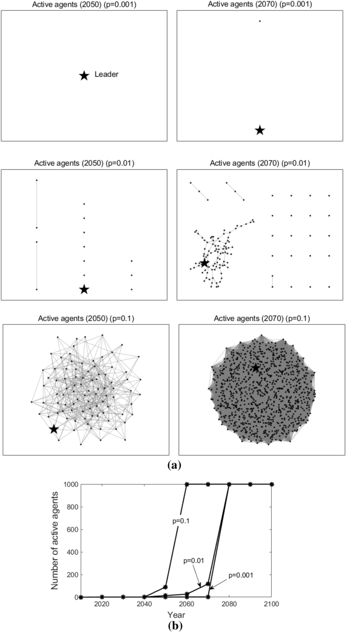
Figure 10 shows the active agents at different times (here we present the active agents in 2050 and 2070 as illustrations) and how the number of active agents changes over time when (p) varies. Likewise, the star-shaped node represents the leader, the black dot nodes represent the followers, and the grey lines represent the edges that connect the agents. As we can observe, when (p = 0.001), in 2050, only the leader adopts T3; in 2070, only one follower starts to adopt T3. When (p = 0.01), in 2050, several followers adopt T3; in 2070, more followers adopt T3. When (p = 0.1), in 2050, about 90 followers start to adopt T3; in 2070, all followers adopt T3. Note that, in the figure, there are independent dot nodes (without the connection to any other nodes). This is because, in our simulation, the random network structure varies at each time t. Previous connected nodes may not be connected currently, but they have already acquired the knowledge of T3 through previous connections. From Fig. 10b), we can conclude that, the higher the connecting probability is, the faster the number of active agents increases, that is, the earlier the followers adopt the new advanced technology T3.

In a word, as the connecting probability (p) increases, more and more followers tend to initiate their adoption of the new advanced technology earlier. It is in accordance with our intuition that with a larger connecting probability, more follower agents could be topologically connected with the leader agent, and they can benefit from the technological spillover effect more straightforwardly.

BA scale-free network

In this subsection, we will run simulations under the assumption that the technological spillover network among all 1000 agents is a BA scale-free network. The ER random graph neglects two most important features of the network in the real world: growth and preferential attachment³⁷.

Following the approach proposed by Albert and Barabási, we construct the scale-free network with the following rules³⁸:

(a)

Initially, there exists a connected network with (m_{0}) nodes. We assume that there are (m_{0} = 10) nodes connecting with each other randomly in the initial network, including the leader Agent 1. The remaining 990 nodes are pending to be added to the network. In each iteration, we add a new node with m edges that link the new node to m present nodes in the system. m should be less than (m_{0}), and we let m = 5.
(b)

When choosing the nodes to which the new node connects, the probability of the new node connecting with a present node i in each iteration is computed with the following equation:

$$begin{array}{*{20}c} {p_{i} = frac{{k_{i} }}{{mathop sum nolimits_{j} k_{j} }},} \ end{array}$$

(8)

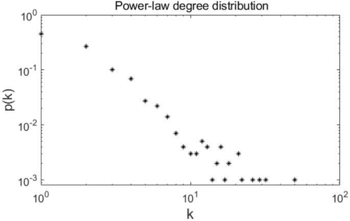
where, (k_{i}) is the degree of present node i, (mathop sum limits_{j} k_{j}) represents the sum of the degrees of all present nodes. Figure 11 shows the power-law degree distribution of the BA scale-free network we constructed.

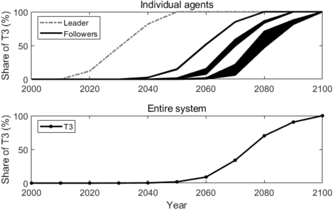
Figure 12 presents how T3 is adopted by individual agents and in the entire system. As we can observe, the followers’ adoption time of T3 ranges from the year 2050 to the year 2080. In the entire system, T3 is adopted around the year 2070, only 10 years earlier compared with what suggested in the reference scenario.

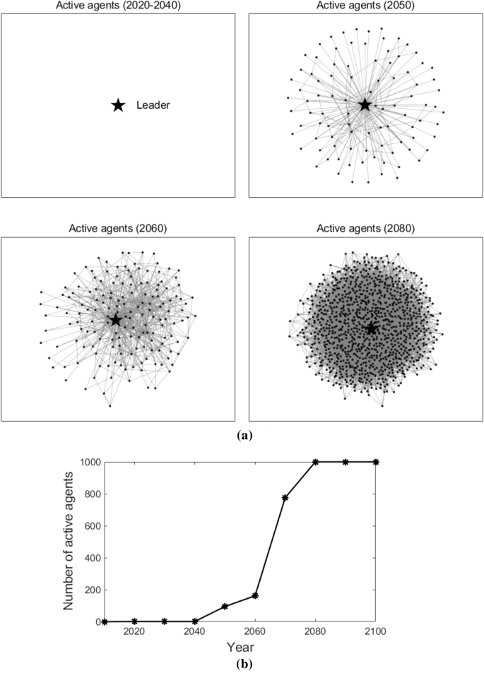
Figure 13 illustrates the active agents at different times and how the number of active agents changes over time in a scale-free network. As we can see, from the year 2020 to 2040, only the leader adopts T3; from the year 2050 to 2070, more and more followers start to adopt T3; and after the year 2080, all the followers adopt T3. This is because, in the scale-free network, most edges are connected to some nodes, i.e., a large number of agents are connected to only some agents, while the other agents are only connected to few agents. Those followers that link directly with the leader will adopt T3 earlier than the followers that are more distant from the leader.

With the discussion above, we can draw the conclusion that, the topological structure of the technological spillover network among agents plays a crucial part in the adoption and diffusion of the new advanced technology among agents and in the entire system. Some network topological structures favor the adoption and diffusion of the new technology (e.g., the globally coupled network), while others may cause adoption time lags among the follower agents (e.g., the random network and the scale-free network), and therefore delay the adoption of the new technology in the entire system. The implication of our simulation is that, in the real world, the network topological structure among decision entities might be complex. It is crucial for the social planner to take into consideration of the network structure when evaluating the diffusion process of an innovation.

In the next section, we will discuss the implication of our research further. We will examine whether different network topological structures influence the effectiveness of a carbon emission constraint policy.

[ad_2]

Source link